GA4 + BigQuery: Month-by-Month Revenue Analysis After User Acquisition

Editor's note: this article was originally published on LinkedIn by Enio Kurteši, and is now released here in its entirety—plus expanded a little in this blog by some additional analysis in Google Sheets, and showing results from a real-life e-commerce dataset for better illustration.

Cohort analysis is a powerful analytical technique that groups customers into "cohorts" based on shared characteristics or experiences within specific time periods. Unlike traditional metrics that provide snapshot views, cohort analysis tracks how these distinct groups behave over time, revealing patterns that might otherwise remain hidden.

For e-commerce businesses, understanding how different customer groups perform over time provides insights that directly impact marketing strategy, product development, and financial forecasting. By tracking groups of customers who started their journey at the same time, businesses can identify patterns that reveal the true health of their customer base and the effectiveness of their acquisition channels.

This time-normalized view reveals patterns and trends that aggregate metrics often obscure, answering critical business questions:

• Are newer cohorts performing better or worse than older ones?
• How does revenue per customer evolve over the customer lifecycle?
• Which acquisition periods yielded the most valuable customers?
• Do seasonal factors affect long-term customer value?

In today’s article, we’ll explore how to analyze revenue by monthly acquisition cohorts, tracking how each group contributes revenue in the months following acquisition using BigQuery.

The SQL Implementation

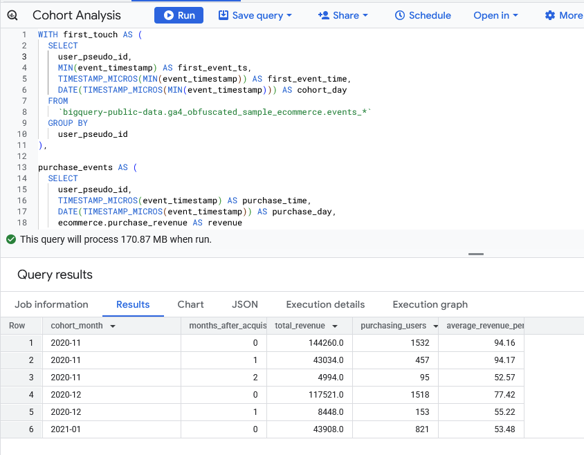
The following BigQuery SQL query provides a solution for cohort revenue analysis using GA4 data:

WITH first_touch AS (
  SELECT 
    user_pseudo_id,
    MIN(event_timestamp) AS first_event_ts,
    TIMESTAMP_MICROS(MIN(event_timestamp)) AS first_event_time,
    DATE(TIMESTAMP_MICROS(MIN(event_timestamp))) AS cohort_day
  FROM 
    `bigquery-public-data.ga4_obfuscated_sample_ecommerce.events_*`
  GROUP BY 
    user_pseudo_id
),

purchase_events AS (
  SELECT
    user_pseudo_id,
    TIMESTAMP_MICROS(event_timestamp) AS purchase_time,
    DATE(TIMESTAMP_MICROS(event_timestamp)) AS purchase_day,
    ecommerce.purchase_revenue AS revenue
  FROM
    `bigquery-public-data.ga4_obfuscated_sample_ecommerce.events_*`
  WHERE
    event_name = 'purchase'
),

cohort_revenue AS (
  SELECT
    ft.user_pseudo_id,
    ft.cohort_day,
    EXTRACT(MONTH FROM ft.cohort_day) AS acquisition_month,
    EXTRACT(YEAR FROM ft.cohort_day) AS acquisition_year,
    pe.purchase_day,
    -- Calculate exact months difference accounting for varying month lengths
    EXTRACT(MONTH FROM pe.purchase_day) - EXTRACT(MONTH FROM ft.cohort_day) + 
    12 * (EXTRACT(YEAR FROM pe.purchase_day) - EXTRACT(YEAR FROM ft.cohort_day)) AS months_after_acquisition,
    pe.revenue
  FROM
    first_touch ft
  JOIN
    purchase_events pe
  ON
    ft.user_pseudo_id = pe.user_pseudo_id
)

SELECT
  FORMAT_DATE('%Y-%m', cohort_day) AS cohort_month,
  months_after_acquisition,
  ROUND(SUM(revenue), 2) AS total_revenue,
  COUNT(DISTINCT user_pseudo_id) AS purchasing_users,
  ROUND(SUM(revenue) / COUNT(DISTINCT user_pseudo_id), 2) AS average_revenue_per_user
FROM
  cohort_revenue
GROUP BY
  cohort_month, months_after_acquisition
ORDER BY
  cohort_month, months_after_acquisition;

Let's break down this query step by step, examining each Common Table Expression (CTE) and its purpose.

CTE 1: first_touch

WITH first_touch AS (
  SELECT 
    user_pseudo_id,
    MIN(event_timestamp) AS first_event_ts,
    TIMESTAMP_MICROS(MIN(event_timestamp)) AS first_event_time,
    DATE(TIMESTAMP_MICROS(MIN(event_timestamp))) AS cohort_day
  FROM 
    `bigquery-public-data.ga4_obfuscated_sample_ecommerce.events_*`
  GROUP BY 
    user_pseudo_id
),

This initial CTE establishes when each user first interacted with the website.

1. Identifies each user via user_pseudo_id
2. Finds their earliest event timestamp using the MIN() function
3. Extracts just the date component for cohort assignment using DATE()

The result is a dataset where each user is assigned to a specific cohort day, the date of their first interaction. This forms the foundation of the entire cohort analysis.

CTE 2: purchase_events

purchase_events AS (
  SELECT
    user_pseudo_id,
    TIMESTAMP_MICROS(event_timestamp) AS purchase_time,
    DATE(TIMESTAMP_MICROS(event_timestamp)) AS purchase_day,
    ecommerce.purchase_revenue AS revenue
  FROM
    `bigquery-public-data.ga4_obfuscated_sample_ecommerce.events_*`
  WHERE
    event_name = 'purchase'
),

The second CTE isolates all purchase events with their associated revenue data:

1. Filters events to include only purchases using WHERE event_name = 'purchase'
2. Captures the purchase timestamp and converts it to a readable format
3. Extracts the purchase date
4. Retrieves the revenue amount from the ecommerce.purchase_revenue field

This creates a dataset of all purchase activity across all users, which will later be joined with the cohort information.

CTE 3: cohort_revenue

cohort_revenue AS (
  SELECT
    ft.user_pseudo_id,
    ft.cohort_day,
    EXTRACT(MONTH FROM ft.cohort_day) AS acquisition_month,
    EXTRACT(YEAR FROM ft.cohort_day) AS acquisition_year,
    pe.purchase_day,
    -- Calculate exact months difference accounting for varying month lengths
    EXTRACT(MONTH FROM pe.purchase_day) - EXTRACT(MONTH FROM ft.cohort_day) + 
    12 * (EXTRACT(YEAR FROM pe.purchase_day) - EXTRACT(YEAR FROM ft.cohort_day)) AS months_after_acquisition,
    pe.revenue
  FROM
    first_touch ft
  JOIN
    purchase_events pe
  ON
    ft.user_pseudo_id = pe.user_pseudo_id
)

This CTE connects users' first-touch data with their purchase history:

1. Joins the first_touch and purchase_events CTEs on user_pseudo_id
2. Extracts the month and year components from the cohort date for easier processing
3. Calculates the number of months between the cohort date and each purchase date

Final SELECT Statement

SELECT
  FORMAT_DATE('%Y-%m', cohort_day) AS cohort_month,
  months_after_acquisition,
  ROUND(SUM(revenue), 2) AS total_revenue,
  COUNT(DISTINCT user_pseudo_id) AS purchasing_users,
  ROUND(SUM(revenue) / COUNT(DISTINCT user_pseudo_id), 2) AS average_revenue_per_user
FROM
  cohort_revenue
GROUP BY
  cohort_month, months_after_acquisition
ORDER BY
  cohort_month, months_after_acquisition;

In the final stage of the analysis, the data is organized into a structured, easy-to-interpret format that highlights revenue trends over time. Each cohort’s acquisition date is reformatted into a simple year-month label (e.g., “2021-03”) for clarity.

The results are then grouped by cohort month and the number of months since acquisition, creating a consistent timeline for comparison. For every month in a cohort’s lifecycle, the analysis sums up the total revenue and counts how many unique users made a purchase.

These figures are used to calculate the average revenue per user, giving a clear view of how customer value develops over time.

The output is arranged chronologically, so you can easily follow each cohort’s performance month by month. The result is a detailed cohort revenue matrix that uncovers long-term patterns and differences across acquisition groups.

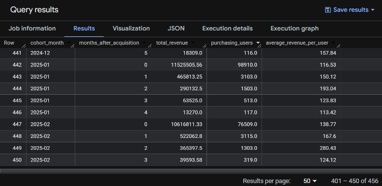
Editor's note: now let's try on a real-life ecommerce dataset, to see what it looks like when we have more data.

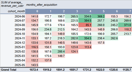
This data—especially when the data spans across many months—is even more useful when visualized in a pivot table. Since the cohort analysis output is always a small table (unless it covers centuries 😆), easiest is to copy the output to the clipboard (Save Results / Copy to Clipboard) and paste it into Google Sheets, and then create a pivot table similar to this:

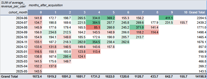
With some conditional formatting, we can see that summer 2024 cohorts were particularly strong, and so was the cohort from last November, while the others, not so much. Everyone starts with a modest value in their first month, but some cohorts "ramp up" nicely over time. Of course, it is best to check if the pattern still holds with the overall volumes as well, but here there are enough customers in each cohort to draw conclusions. Also, in some businesses, Black Friday and Christmas (and seasonality in general) could distort certain months, which has to be considered when drawing conclusions. All that said, these patterns can now be cross-checked with campaigns, promotions and other activities to explain the different behaviors by various cohorts.

Conclusion

Cohort analysis by acquisition month offers a powerful way to understand how customer behavior and revenue evolve over time.

This approach answers key questions like:

1. Are recent customers spending more or less than those acquired in previous months?
2. How quickly does revenue ramp up after acquisition?
3. And how does long-term customer value compare across different marketing periods?

By isolating each cohort and analyzing their spending habits in the months following acquisition, businesses gain a much clearer picture of customer retention, engagement, and lifetime value. This insight is especially valuable for optimizing marketing spend, improving onboarding, and identifying high-performing acquisition periods. For example, if users acquired in March consistently generate more revenue over six months than those from other months, it might signal a particularly effective campaign or seasonal advantage worth repeating.

We’d love to hear your thoughts, drop a comment and let us know how you're using cohort analysis in your own work, or if you have questions about implementing it!

Thanks for reading! 😊